E. Marguí,a,* M. Hidalgoa and I. Queraltb
aDepartment of Chemistry. University of Girona. Campus Montilivi, 17071 Girona, Spain
bInstitute of Earth Sciences “Jaume Almera”, CSIC, C/Lluis Sole Sabaris s/n, 08028 Barcelona, Spain
Introduction
The use of vegetation specimens as bioindicators of the degree of pollution with metallic elements in environmental monitoring studies is widespread. In such studies, conclusions are drawn on the basis of an examination of a large number of samples. Hence, it is important that the analytical procedures used should be rapid and simple, without detriment to appropriate accuracy and precision in analyte concentration determination.
Atomic spectrometry is the most obvious choice of technique to be used for metal determination in these kinds of samples.1 The basic instrumentation is, however, designed for the analysis of liquid samples. Therefore, solid samples have to be brought into solution in order to satisfy the needs of sample introduction systems for most of the atomic spectroscopic techniques used. For some types of samples, dissolution is not a problem and it may be readily achieved using mixtures of strong acids (generally nitric and sulphuric) and oxidants (commonly hydrogen peroxide). However, plant samples often require a more complete decomposition procedure to ensure efficient solubilisation of metals into solution due to the presence of high contents of silicon. Most of the usual wet methodologies proposed rarely include means to overcome the particular silicon problem and this leads to poor recoveries of some elements, because of the analyte binding with the insoluble residue.2 For such cases, an additional hydrofluoric acid attack and evaporation to dryness is necessary to ensure a complete dissolution of the analytes.3 The large numbers of acid mixtures in wet ashing procedures that have been proposed in the literature illustrate the fact that a lack of a consensus exists for plant specimen dissolution. In most cases, the choice of the best decomposition procedure for vegetation samples involves the evaluation of the procedure for each specific matrix and each analyte under study. This becomes unfeasible in environmental studies where several plant species are used as pollution indicators of different heavy metals. In view of these problems, the implementation of other methodologies that allow for avoiding the matrix destruction stage has increased over the last few years.
Most of the X-ray Fluorescence (XRF) techniques comply with the desired features for the analysis of vegetation specimens, including: (i) the possibility to perform the analysis directly on solid samples, (ii) multi-element capability, (iii) the possibility to perform qualitative, semi-quantitative and quantitative determinations, (iv) a wide dynamic range, (v) high throughput and (vi) low cost per determination. The main drawbacks of XRF instrumentation, restricting more frequent use of the technique for environmental purposes, have been its limited sensitivity for some important pollutant elements (such as Cd and Pb, among others) and a somewhat poorer precision and accuracy compared to other atomic absorption spectroscopic techniques. Nevertheless, recent improvements in the XRF instrumentation, such as the development of digital signal processing based spectrometers in combination with enhanced X-ray production using better designs for excitation–detection, has added the advantage of increasing instrumental sensitivity, thus allowing the improvement of both precision and productivity. This has promoted an increasing interest in using X-ray fluorescence spectroscopy in the environmental analysis field as an alternative to destructive analytical methods. In particular, the implementation of different quantification strategies using different configurations of XRF spectrometers as analytical tools to determine chemical composition of vegetation matrices is outlined in this article.
Detailed information and results about this topic are described in full in previously published papers.2,4,5
Sample preparation for XRF analysis
To study the applicability of XRF for trace element analysis of vegetation samples in environmental studies, some higher (vascular) plants (Betula pendula, Buddleia daviddii, Quercus robur and Pinus sylvestris), grasses (Bromus sp.) and mosses (Leucobyum sp. and Pleurocarpus sp.) growing on the waste landfills of different abandoned Pb–Zn mining areas in Spain were collected.
Once at the laboratory, vegetation samples were washed thoroughly with deionised water to remove superficial dust and oven-dried at 55 ± 5°C for 24 hours. To reduce particle size and satisfy the conditions for homogeneity, they were ground in an agate ball mixer mill using a grinding time in the range 2–5 min. Once plant tissues were powdered and dried, they were kept in capped polypropylene flasks until analysis.
As mentioned before, an advantageous feature that makes XRF techniques attractive alternatives to destructive analytical methods is the possibility of performing the analysis directly on solid samples. This advantage usually implies a simpler sample preparation with a considerable reduction of reagents and risk of contamination.
The methodology used in the present study consisted of weighing 2 g of powdered sample (without the addition of a binder) and pressing it at 20 tons cm–2 for 60 s to obtain a cylindrical pellet of 20–40 mm diameter. Then, each pellet was placed on a sample holder and located directly in the X-ray beam of the X-ray spectrometer used for elemental determination.
XRF instrumentation
There are many types of XRF spectrometers available on the market today, most of which can be separated roughly into two categories: wavelength dispersive X-ray fluorescence (WDXRF) and energy dispersive X-ray fluorescence (EDXRF).
In WDXRF, the characteristic radiation emitted from the sample is separated into wavelengths using a diffraction device [see Figure 1(a)]. Usually in WDXRF spectrometers, the analysis of different elements is carried out in a sequential way by scanning synchronously the orientation of the monochromator device and the detector (2θ). Whereas, in multi-channel spectrometers, the use of several diffraction devices/detectors set-ups allows one to measure several elements simultaneously (the number of channels is, however, limited).
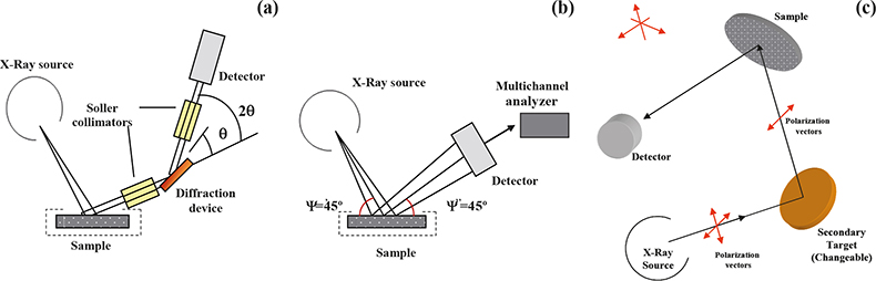
Figure 1. Configuration of the XRF spectrometers used. (a) Conventional WDXRF spectrometer. (b) Conventional EDXRF spectrometer. (c) Polarised-beam EDXRF spectrometer.
Unlike the wavelength dispersive X-ray fluorescence systems, conventional EDXRF spectrometers consist of only two basic units, the excitation source and the spectrometer/ detection system [see Figure 1(b)]. In this case, the resolution of the energy dispersive system is equated directly to the resolution of the detector, typically a semiconductor detector of high intrinsic resolution is employed [Si (Li)]. The use of this type of detector allows one to record an electronic signal, the current of which is proportional to the energy of the detected photon. Then a multi-channel analyser is used to collect, integrate and display the resolved pulses. It is interesting to remark that using this configuration, all of the X-rays emitted by the sample are collected at the same time (simultaneously measured), giving great speed in the acquisition and display of data. In practice, however, there is a limit to the maximum count rate that the spectrometer can handle and this led, in the mid-1970s, to the development of the so-called secondary mode of operation. In the secondary mode, a carefully selected pure element standard (secondary target) is interposed between the primary source and the sample in such a way that a selectable energy range of secondary photons is incident upon the sample. This geometry (called tri-axial) reduces the background radiation relative to the characteristic radiation from different elements in the sample, allowing an improvement in the sensitivity and limits of detection of minor and trace elements. With novel instrumentation [polarised-beam EDXRF (EPDXRF)] the combination of polarisation (tri-axial geometry) with the possibility of using different secondary sources allows for specific element excitation and, thus, a further improvement of the limits of detection of analytes [see Figure 1(c)]. Another advantage of scattering primary X-rays with targets is that it is much more practical to vary targets than X-ray tube anodes, and targets may be used to produce fluorescence lines to act as near-monochromatic secondary sources at slightly higher energies than the absorption edges of the analytical lines to be excited. By combining polarisation with the possibility of different secondary sources, an instrument can be designed to generate a range of excitation and polarisation conditions optimised for different groups of analytes.
In the present work, three configurations of XRF spectrometers were used [WDXRF, EDXRF and high-energy polarised-beam dispersive XRF (EDPXRF)] to study their possibilities and limitations for elemental determination in vegetation matrices. In Table 1 the main instrumental parameters for each configuration are displayed, including the excitation mode of operation and acquisition time, which was selected as a trade-off between an acceptable repeatability of measurements and total analysis time.
Table 1. Instrumental parameters for the X-ray fluorescence spectrometers used.
XRF configuration | Elements | Instrument characteristics | Excitation | Acquisition time |
EDPXRF | K, Ca, Mn, Fe, Cu, Sr, Pb, Zn | X-ray tube | Primary X-ray beam scattered by a secondary target (Mo) | 1000 s (total) |
WDXRF | Na, Mg, Al, P, S, K, Ca, Mn, Fe, Co, Zn, As, Sr, Pb | X-ray tube | Primary X-ray beam | 100 s (Co, Zn,Pb) |
High-energy EDPXRF | Cd, Pb, As, Cu, Fe, Zn | X-ray tube | Primary X-ray beam scattered by changeable secondary targets (Cd: Al2O3, Pb: Zr, Others: KBr) Polarised X-ray beam (tri-axial geometry) | 1000 s (Cd) |
Notes: Instrumentation: EDXRF: non-commercial equipment, Centro de Fisica Atomica, Universidade de Lisboa, Portugal. WDXRF: S4 Explorer, Bruker. EDPXRF: Epsilon5, PANalytical. Crystals: OVO-55 (W/Si multilayer), PET (Pentaerythrite), LiF200 (Lithium fluoride). Detectors: FPC (flow proportional counter), SC (scintillation counter).
Quantitation methods
In general, XRF quantitative analysis is carried out by the calibration curve method, generated from measurements made with many calibration standards. However, for some applications (such as plant specimens) it is difficult to get sufficient certified standards, with similar matrices to the samples, in order to achieve a good spread of data points over the range of each element to be determined. In such cases, the use of standard-less quantitative procedures based on the Fundamental Parameter (FP) algorithm are commonly applied.6 However, the use of standards prepared in the laboratory with commercially available pure elements or compounds has been shown to be efficient for calibration purposes since they are inexpensive and can be easily prepared. Plant material consists mainly of C, N, H and O (cellulose matrix). Accordingly, the use of several synthetic standards made of cellulose could provide a good means to simulate the vegetation matrix and obtain reliable calibration curves with a good spread of data points over the range of each element to be determined.
In the case of vegetation samples, the absorption of the measured X-rays by the matrix is relatively small compared to other heavier samples (i.e., rock or soil samples). Nevertheless, due to the widely variable range of concentrations of K, Ca, Cl and other elements in plant samples, in most cases, correction for the matrix effects is necessary in order to obtain quantitative results. Several methods have been described for matrix effect corrections including the use of influence coefficients.
In Table 2 the quantitative approaches used in each instrument configuration are summarised and in Figure 2 two examples of calibration curves are displayed for the analysis of minor (Fe) and trace (Cd) elements in vegetation matrices.
Table 2. Summary of the performance of XRF analysis of vegetation samples.
XRF configuration | Quantitative analysis | Limits of detection (mg kg–1) | Relative precision (%) | Relative bias (%) | Observations |
EDPXRF | FP | K= 10.0, Ca = 20.0, Mn = 4.0, Fe = 3.1, Cu = 1.2, Zn = 1.2, Sr= 1.1, Pb = 1.1 | (NIST SRM 1571) | (NIST SRM 1571) |
|
WDXRF | ECC (synthetic cellulose standards) | Na = 80, Mg = 50, Al = 30, P= 30, S= 40, K= 400, Ca = 200, Mn = 6, Fe = 20, Co = 0.5, Zn = 5, As = 1, Sr= 0.7, Pb = 6 | (GBW 07602) | (GBW 07602) |
|
High-energy EDPXRF | ECC (Cd) | Pb = 0.27, Zn = 0.18, Fe = 0.58, As = 0.20, Cu = 0.24, Cd = 0.7 | (GBW 07602) | (GBW 07602) | Cd (Kα line) Interference of As-Kα and Pb-Lα was solved by employing selective excitation with targets of different materials |
Notes: ECC: Empirical calibration curve, FP: Fundamental parameters approach (standard-less). Relative precision = (St. Dev / Average) × 100. Relative bias = [(Average-certified)/certified] × 100. NIST SRM 157: [K] = 1.47 ± 0.03%, [Ca] = 2.09 ± 0.03%, [Mn] = 91 ± 4 mg kg–1, [Fe] = 300 ± 20 mg kg–1, [Cu] = 12 ± 1 mg kg–1, [Zn] = 25 ± 3 mg kg–1, [Sr] = 37 ± 1 mg kg–1, [Pb] = 45 ± 3 mg kg–1. GBW07602: [Na] = 1.10 ± 0.06%, [Mg] = 0.287 ± 0.011%, [Al] = 0.214 ± 0.018%, [P] = 0.083 ± 0.003%, [S] = 0.32 ± 0.02%, [K] = 0.85 ± 0.03%, [Ca] = 2.22 ± 0.07%, [Mn] = 58 ± 3 mg kg–1, [Fe] = 1020 ± 40 mg kg–1, [Co] = 0.39 ± 0.03 mg kg–1, [Zn] = 20.6 ± 1 mg kg–1, [As] = 0.95 ± 0.08 mg kg–1, [Sr] = 345 ± 7 mg kg–1, [Pb] = 7.1 ± 0.7 mg kg–1, [Cu] = 6.6 ± 0.4 mg kg–1. NIST SRM 1570a: [Cd] = 2.89 ± 0.07 mg kg–1.
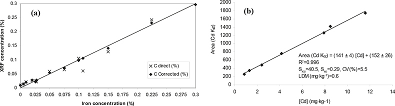
Figure 2. Calibration curves obtained for a minor element, Fe (a), and for a trace element, Cd (b). (a) WDXRF: synthetic cellulose standards; matrix correction: influence coefficients. (b) High-energy EDPXRF: secondary standards (vegetation samples previously analysed by ICP-MS).
Results
In order to study the capability of the proposed analytical procedures for the intended purpose, the evaluation of some analytical figures of merit including limits of detection, precision and accuracy was carried out throughout the analysis of different certified reference plant materials (see Table 2).
Data obtained showed up the benefits of using polarised X-ray sources (primary beam scattered by a secondary target) to reduce the characteristic high degree of scattering of the X-ray source by vegetation matrices leading to an improvement in the limits of detection. The application of an EDXRF analytical methodology based on this configuration allowed the quantification of eight elements (K, Ca, Mn, Fe, Cu, Zn, Sr and Pb) at mg kg–1 levels with a precision <8% for all elements and in most cases <5%, similar to those obtained by other atomic spectroscopic techniques.
For WDXRF, in spite of achieving similar precisions in the obtained data, poorer detection limits were obtained compared to the EDXRF methodology mentioned above, especially for heavier elements. Nevertheless, by means of WDXRF the determination of most light elements was somewhat better.
Finally, improved instrumental sensitivity and detection limits (low mg kg–1 range) for the determination of several trace elements (Cd, Pb, As, Cu, Fe and Zn) in vegetation matrices was achieved by using EDPXRF. In this case, the combination of selective excitation (using different secondary targets), polarised X-ray beam, the use of a gadolinium X-ray tube and a high-energy detector overcomes the problems of reduced sensitivity and spectral interferences inherent in the choice of Lα lines for the determination of heavy metals, commonly used in conventional XRF instrumentation. Therefore, the determination of some important pollutant elements such as cadmium was feasible in the low mg kg–1 range.
After the validation process, the XRF technique was applied to the analysis of different vegetation species to evaluate the environmental effects of metal dispersal around abandoned Pb–Zn mining areas in Spain.7
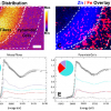
Results obtained from the analysis of 38 vegetation samples are shown in Figure 3(a). It can be observed that the highest concentrations found in all the species studied correspond to Zn, Pb and Fe, which were the main metals extracted from the ore vein of the mining districts studied. In addition, significant concentrations of minor metals such as Cd and As are also present in the vegetation specimens, being the largest in the case of moss species (Leucobryum sp., Pleurocarpus sp.) and grasses (Bromus sp.) with values up to 28 mg kg–1 and 3 mg kg–1 for Cd and As, respectively.
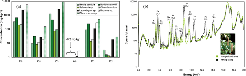
Figure 3. Application of XRF for the analysis of vegetation samples contaminated by mining activities. Comparison of average metal content for all species studied at different sites around the mining districts studied (high-energy EDPXRF). Spectra obtained with EDXRF analysis on leaves (Betula pendula) collected on a mining landfill with the corresponding content in a specimen sampled far from the mining activities (control sample).
In Figure 3(b), a representation of two measured spectra obtained with EDXRF analysis on leaves of Betula pendula is displayed. At a cursory glance, the spectra allow discrimination between a sample growing on a mining waste landfill site from one sample growing far from the mining activities (control sample), corroborating the metal accumulation process occurring in vegetation. These results prove the risk that abandoned mining districts represent for the biota in these areas.
Summary
Data obtained highlighted that XRF spectrometry could be a good analytical tool for trace metal analysis of vegetation samples as an alternative to classical destructive methods, given that it provides accuracy and precision fulfilling the requirements for environmental studies. Moreover, this method is less time consuming, requires less amounts of reagents and it is easy to control, because it almost does not require supervision. This is of great importance in environmental studies where conclusions are based on the analysis of a large number of samples.
It is expected that future improvements in XRF instrumentation should increase, even more, the instrumental sensitivity and, thus, XRF spectrometry could offer new possibilities in the environmental field in the future.
Acknowledgements
A significant part of the experimental work has been developed in the “Departamento de Física, Universidade de Lisboa (Portugal)” and in the “Micro and Trace Analysis Center (MiTAC), Department of Chemistry, University of Antwerpen (Belgium)”. Therefore, the authors wish to thank to Maria Luisa de Carvalho Leonardo, Professora do Centro de Física Atómica da Universidade de Lisboa, and Professor René Van Grieken, director of MiTAC, for the major contributions and continuous support supplied.
The dedicated work of Roman Padilla Álvarez, belonging to the Centre of Technological Applications and Nuclear Development (CEADEN, Havana, Cuba) was essential for the successful investigations.
This study was financed by the Spanish National Research Programme (Ref. CGL2004–05963-C04–03/HID).
References
- C. Baffi, M. Bettinelli, G.M. Beone and S. Spezi, Chemosphere 48, 299 (2002).
- E. Marguí, I. Queralt, M.L. Carvalho and M. Hidalgo, Anal. Chim. Acta 549, 197 (2004).
- M. Hoeing, Talanta 54, 1021 (2001).
- E. Marguí, M. Hidalgo and I. Queralt, Spectrochim. Acta Pt B Atom. Spectr. 60, 1363 (2005).
- E. Marguí, R. Padilla, M. Hidalgo, I. Queralt and R. Van Grieken, X-Ray Spectrom. 35, 169 (2006).
- R. Van Grieken and A.A. Markowicz (Eds), Handbook of X-Ray Spectrometry. Methods and Techniques. Marcel Dekker, Inc. (1993).
- E. Marguí, Analytical methodologies based on X-Ray fluorescence spectrometry (XRF) and inductively coupled plasma spectroscopy (ICP) for the assessment of metal dispersal around mining environments. Doctoral Thesis, Girona, Spain (2006).