The variographic experiment

Kim H. Esbensen^a and Claas Wagner^b

^aKHE Consulting, www.kheconsult.com
^bSampling Consultant—Specialist in Feed, Food and Fuel QA/QC. E-mail: [email protected]

Pierre Gy, the inventor of the Theory of Sampling (TOS), pioneered applications of variography to understanding large-scale variability in process plants and process control from as early as the 1950s and devoted a major part of his TOS development period to this subject. The variogram allows one to identify sources of variability and provides valuable insight into correlations between successive samples. Neglect or poor understanding of the data analytical capabilities of the variogram means that it has not been widely applied in process control until now, except in industry sectors which have embraced TOS (mining, cement and certain parts of the process industries) because of the overwhelming consequences of making wrong decisions when treating vast tonnages—the consequences of wrong decisions are simply too great. Failure to address stream heterogeneity means that conventional statistics and Statistical Process Control (SPC) too often fail to identify and distinguish the true sources of variability in a process stream. For each type of heterogeneity, there is a matching variety of process variability. Although the method is powerful in terms of the insights one is able to gain in regard to plant performance and management, examples of the application of this particular method have been suspiciously little notable in the literature.

The variogram

Any process stream or similar that are to be sampled should always first be subjected to a “variographic experiment”, the purpose of which is to tune in an optimised sampling frequency based on the increment size selected. The variographic experiment will also allow estimation of an optimal number of increments to be aggregated as composite samples. It is the responsibility of the sampler to come up with the best possible initial suggestion for the size of the increments to be used; obviously previous experience and knowledge regarding the specific process at hand are of premium value in this endeavour.

In order to characterise a process stream, it is necessary to extract a certain number of increments, N_U, to have these analysed in the laboratory and to conduct calculations based on the variographic master equation, Figures 1 and 2. The total number of analytical results (stemming from the N_U increments) must be between 60 and 100—it may well be larger (this is actually not such a harsh demand, when it is factored in that most of the variographic characterisations used extensively in science, technology and industry are usually realised based upon automated sampling). In general, it must not be smaller than 60, although very experienced operators occasionally cite the canonical number 42 (however, this is not recommended at large without considerable experience).

Figure 1. Based on a relevant problem-dependent sampling frequency, 60–100 increments need to be extracted (completely TOS-correct). In the specific example shown here the sampling frequency is 2 min.

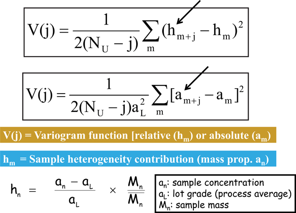
Figure 2. Variogram master equation, expressed both in terms of analytical results, a_m, or alternatively, in terms of the corresponding heterogeneity contributions h_m (the latter was defined in an earlier column, but repeated here for easy reference).

The sampling frequency used in the variographic experiment is either set by the process situation at hand (existing, proven knowledge), or it may be calculated as the total process interval under investigation divided by 60 (or 100). Often there are special circumstances that fix this issue, for example in the case where the variographic experiment is aimed at investigating a current situation, which has an already set sampling frequency. This may be defensible, or it may not—a matter that will be revealed by proper interpretation of the variogram results (lots of examples to follow in subsequent columns).

There may, thus, be many objectives behind a variographic characterisation but all involve deciding upon the most relevant sampling frequency from which to gain a maximum of insight (more on these initiating issues after a first familiarity with the variographic experiment has been gained).

There is, thus, a minimum resolution limit associated with every variographic experiment; there can be no information gained at a scale less than the experimental sampling rate (2 minutes in the example in Figure 1).

The distance between two data points is called the lag, j. The minimum distance between any two data points is termed Θ_min. Any distance between pairs of data points, j, is always referred to the root Θ_min, and will therefore always be a multiplum of Θ_min [j = 1, 2, 3, ..., N_U – 1]. This allows use of a general lag parameter, j, which is independent of the particular measurement unit used. This general lag parameter is a most welcome feature, allowing comparison between variograms of any process, type, material etc. As shall be shown this makes comparative variographic analysis indispensable in process technology and process sampling.

It is often recommended to over-sample for the purpose of the variographic experiment, but we shall temporarily set aside these initiating issues until after an initial familiarity with the variographic experiment has been gained. Thus, in Figure 1 the current sampling frequency was actually ~8 min, but it was decided to over sample by a factor of ×4, because there was a suspicion that the current frequency was actually too high.

The primary job for variographic characterisation, Figures 3 and 4 is to express the variability of the set of N_U analytical results. Remember that due diligence (TOS correctness) must always be observed regarding extraction of all increments (see previous column). Indeed, the same adherence to TOS’ principles is to be observed for all sub-sampling and sample preparation in the lab. On this basis, the only variability left is that between analytical results in the extension dimension (the process dimension). Thus, the variogram is a powerful characterisation of the longitudinal heterogeneity of the process interval under consideration (all transverse heterogeneity w.r.t. the process translation direction has been covered, i.e. incorporated in each increment extracted). N.B. Although in a variographic experiment it is increments which are extracted, they are at first treated as fully competent samples in their individual, own right. The result of a variographic experiment may subsequently result in a certain number of increments being aggregated, see further below. This minor apparent ambiguity need not lead to confusion, however, as soon as the full role and function of a variographic characterisation is comprehended.

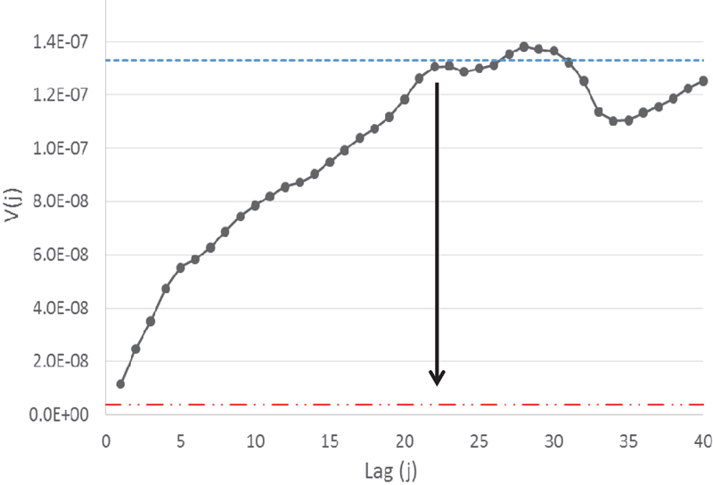
Figure 3. A generic variogram based on 80 increments. Real-world variogram. The lag axis of a variogram will always be of length N_UM/sub> / 2. This particular variogram shows a very small nugget effect (red horizontal line); the sill is marked with a blue line. The range is of the order of 22–23 lags. Note that it is also known from earlier studies of longer duration than the present, that the sill corresponds to the level shown here; this is an example of bringing in full domain-specific knowledge and experience in “reading a variogram”.

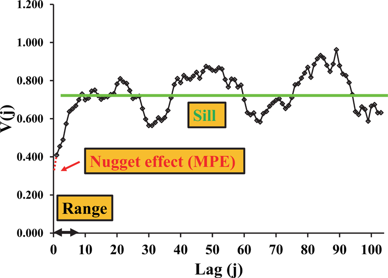
Figure 4. An experimental variogram from a process of great significance in technology and industry, mixing. Note that the original data series is larger than 200 increments.

The variogram principle is to calculate the sum of all squared differences between all pairs of data points with in-between spacing equal to the lag, j, as j spans the entire interval of interest. Thus, the fundamental calculation is repeated for all j lags, i.e. [j = 1, 2, 3, ..., N_U – 1].

Figure 1 shows the spatial disposition of all possible pairs of data pairs as a function of the increasing lag [j = 1, 2, 3, ..., N_U – 1].

The master equation returns one value, the variance V as a function of the lag, V(j), i.e. there is calculated one variance measure corresponding to each lag. The variographic function thus characterises the set of data (in the present process, a time series) by the variance of a set of squared deviations, “one scale at the time” [j = 1, 2, 3, ..., N_U – 1]. Plotting V(j) [Y-axis] as a function of the lag j [X-axis] then produces the variogram, Figures 3 and 4.

There is an apparent ambiguity regarding whether to express the variogram based on absolute concentration values, or recalculated as heterogeneity contributions. Figure 2 shows both options, termed the absolute vs the relative variogram, respectively. This is a matter of no consequence, however, as the shape of the alternative variograms will be identical, with only the unit of measurements (and thus the unit on the Y-axis) differing. Every interpretation of both types of variograms will be identical. The advantage of using the relative variogram is significant, however, as it allows direct comparison of all variograms inter alia, including the levels and magnitudes of ranges, sills and nugget effects.

Based on the present and the preceding two columns, we are now ready for the promised bonanza of real-world examples and case histories from which to learn of the powerful capabilities of variograhics.

Figure 4 is a real world variogram from a technological process, from which several general issues can be learned. The sill is always considered as a kind of ceiling for the total variability across the full lag spectrum—technically, however, the sill is defined as the average variance for all lags. In well-prepared variograms with a sufficient number of increments, the range will usually only constitute a small number of lags, the average variance will occupy exactly this ceiling disposition (note that the ceiling will not cap the variability from above, but from below, being lowered somewhat by the smaller variance levels below the range, made especially clear in Figure 3).

As soon as the lag distance goes beyond the range, the particular variogram in Figure 4 shows a tell-tale periodic disposition with a period of ~30 lags, or slightly higher. The process being characterised is the output of a mixing process which is supposed to have been fully mixed at this stage. The empirical evidence in Figure 4 is interesting in this context as it shows beyond doubt that this objective has not been met—on the contrary there is solid evidence of a systematic compositional periodicity, which is an inheritance from inefficient mixing. This is a role model interpretation of a variogram. Were the mixing process fully efficient there would be no periodicity observable in the output variogram.

There are many other potential gains to be had from proper interpretation of variograms, for example regarding the specific sill level and the magnitude of the nugget effect w.r.t. the sill level, all to be explored in the next columns. Stay tuned—this is where sampling becomes immensely powerful.

As always, should the reader have become seriously impatient, we end with a set of in-depth publications exposing the features treated here more fully. Enjoy!

References

1. K. Engström and K.H. Esbensen, “Evaluation of sampling systems in iron ore concentrating and pelletizing processes – Quantification of Total Sampling Error (TSE) vs. process variation”, J. Mining Eng. in press (2017).https://doi.org/10.1016/j.mineng.2017.07.008
2. E. Thisted and K.H. Esbensen, “Improvement practices in process industry – the link between process control, variography and measurement system analysis”, TOS forum 7, 20–29 (2017). doi: https://doi.org/10.1255/tosf.97
3. E. Thisted, U. Thisted, O. Bøckman and K.H. Esbensen, “Variographic case study for designing, monitoring and optimizing industrial measurement systems – the missing link in Lean and Six Sigma”, in Proc. 8^th International Conference on Sampling and Blending, 9–11 May 2017, Perth, Australia, pp. 359–366 (2017). ISBN: 978 1 925100 56 3
4. R.C.A. Minnitt and K.H. Esbensen, “Pierre Gy’s development of the Theory of Sampling: a retrospective summary with a didactic tutorial on quantitative sampling of one-dimensional lots”, TOS forum 7, 7–19 (2017). https://doi.org/10.1255/tosf.96
5. K.H. Esbensen, A.D. Román-Ospino, A. Sanchez and R.J. Romañach, “Adequacy and verifiability of pharmaceutical mixtures and dose units by variographic analysis (Theory of Sampling) – A call for a regulatory paradigm shift”, Int. J. Pharmaceut. 499, 156–174 (2016). https://doi.org/10.1016/j.ijpharm.2015.12.038
6. K.H. Esbensen and R.J. Romañach, “Proper sampling, total measurement uncertainty, variographic analysis & fit-for-purpose acceptance levels for pharmaceutical mixing monitoring”, in Proceedings of the 7^th International Conference on Sampling and Blending, 10–12 June, Bordeaux, TOS forum 5, (2015). https://doi.org/10.1255/tosf.68
7. A. Sánchez-Paternina, A. Román-Ospino, C. Ortega-Zuñiga, B. Alvarado, K.H. Esbensen and R.J. Romañach, “When “homogeneity” is expected—Theory of Sampling in pharmaceutical manufacturing”, in Proceedings of the 7^th International Conference on Sampling and Blending, 10–12 June, Bordeaux, TOS forum 5, 67–70 (2015). https://doi.org/10.1255/tosf.61
8. Z. Kardanpour, O.S. Jacobsen and K.H. Esbensen, “Local versus field scale heterogeneity characterization – a challenge for representative field sampling in pollution studies”, Soil 1, 695–705 (2015). https://doi.org/10.5194/soil-1-695-2015
9. H. Tellesbø and K.H. Esbensen, “Practical use of variography to find root causes to high variances in industrial production processes – I. Exclay (LECA)” in 6^th World Conference on Sampling and Blending (WCSB6), Lima, Peru, 19–22 November 2013, pp. 275-286. http://www.gecaminpublications.com/articulos/wcsb613_c0605_telesbo.pdf_4896205081.pdf
10. H. Tellesbø and K.H. Esbensen, “Practical use of variography to find root causes to high variances in industrial production processes – II. Premixed mortars”, in 6^th World Conference on Sampling and Blending (WCSB6), Lima, Peru, 19–22 November 2013, pp. 287–294. http://www.gecaminpublications.com/articulos/wcsb613_c0606_telesbo.pdf_9420653199.pdf
11. K.H. Esbensen, C. Paoletti and P. Minkkinen, “Representative sampling of large kernel lots – I. Theory of Sampling and variographic analysis”, Trends Anal. Chem. 32, 154–165 (2012). https://doi.org/10.1016/j. trac.2011.09.008
12. P. Minkkinen, K.H. Esbensen and C. Paoletti, “Representative sampling of large kernel lots – II. Application to soybean sampling for GMO control”, Trends Anal. Chem. 32, 166–178 (2012). https://doi.org/10.1016/j.trac.2011.12.001
13. K.H. Esbensen, C. Paoletti and P. Minkkinen, “Representative sampling of large kernel lots – III. General considerations on sampling heterogeneous foods”, Trends Anal. Chem. 32, 179–184 (2012). https://doi.org/10.1016/j.trac.2011.12.002
14. F.F. Pitard, Pierre Gy’s Sampling Theory and Sampling Practice: Heterogeneity, Sampling Correctness and Statistical Process Control, 2^nd Edn. CRC Press (1993). ISBN: 0-8493-8917-8
15. P. Gy, Sampling for Analytical Purposes, 2^nd Edn, Translated by A. Royle. John Wiley, Chichester (1999).