N.M. Faber,a,* F.H. Schreutelkampb and H.W. Vedderc
aChemometry Consultancy, Rubensstraat 7, 6717 VD Ede, The Netherlands
bAbbott International, Quality Assurance, Rieteweg 21, 8041 AJ Zwolle, The Netherlands
cBlgg Oosterbeek, Mariendaal 8, PO Box 115, 6860 AC Oosterbeek, The Netherlands
There is little profit in approximations which are good but not known to be good.
B.N. Parlett, The Symmetric Eigenvalue Problem (1980)
Introduction
The goal of building a multivariate calibration model is to predict a chemical or physical property from a set of predictor variables, e.g. analyte concentration or octane number from a near infrared (NIR) spectrum. A good multivariate calibration model should be able to replace the laborious, possibly imprecise reference method. The quality of a model therefore primarily depends on its predictive ability. Other properties such as interpretability of the model coefficients might also be of interest, but here the focus is on the problem of quantifying the predictive ability. Note that this problem is solved for univariate calibration based on least-squares straight-line fitting because standard expressions can be used to calculate prediction intervals (Figure 1). Unfortunately, multivariate calibration is much more complex owing to the richer data structures involved and the large variety of estimation procedures available. Here we will restrict ourselves to model building using partial least squares regression (PLSR), since it is the de facto standard in chemometrics. Because generally agreed expressions for multivariate prediction intervals do not exist, one usually combines the observed prediction errors for an independent test set in a standard error of prediction (SEP). This summary statistic is then used as an approximation of the standard deviation of the prediction error for all future prediction samples. However, this average prediction error estimate cannot be used to construct prediction intervals as displayed in Figure 1 for the obvious reason that it is a constant.
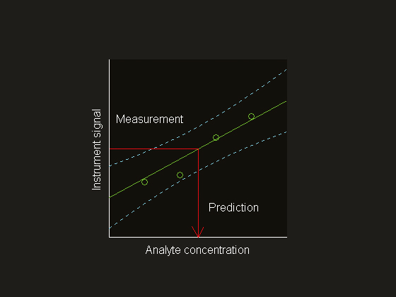
Figure 1. Univariate instrument signal versus analyte concentration. The model (—) is based on the measurement for four samples (o). The dashed lines (---) are the 95%prediction bands that connect the prediction intervals for each value of the instrument signal. The prediction intervals are smallest close to the model centre, where the model is most precise.
Recently, important advances have been reported with respect to estimation of multivariate SEP. A clear distinction can be made in terms of their intended scope: while DiFoggio1 and Sørensen2 improve estimation of SEP on the global set level, Fernández Pierna et al.3 claim to achieve this on the individual sample level. The latter contribution can therefore be seen as an attempt to reduce the gap between univariate and multivariate calibration methodology. The purpose of the current paper is to illustrate the internal consistency of these contributions. This consistency directly follows from a comparison of relatively simple mathematical formulae. The main point to be learned from these formulae is the confusing role of the uncertainty in the reference values used for model building and testing.
Example data set
Fearn4 published a NIR data set that was collected for the prediction of % protein in ground wheat samples. The reference values were obtained using the Kjeldahl method, which has an estimated standard deviation of 0.2% at 10% protein. The calibration and test sets consist of 24 and 26 samples, respectively. The NIR reflectance spectra are digitised at six different wavelengths in the range 1680–2310 nm. This data set has been used extensively in the chemometrics literature for method testing. Mean centring has been applied before PLSR modelling. Cross-validation has been employed for factor selection and it was concluded that the optimum model requires four factors (see Figure 2). A principal component analysis of the mean-centred spectra reveals that test sample 1 deviates from the rest of the population. This can be visualised by plotting the normalised scores (Figure 3). The results for the fourth principal component indicate that this sample is much further away from the mean of the calibration set data than are the others. Plotting principal component scores is often more informative than plotting the spectra themselves. In this case, the mean-centred spectra do not give a clear indication of why this test sample should be abnormal (see Figure 4). It is important to note that extreme test samples are very useful in the current context, namely prediction uncertainty estimation on both the global set as well as the individual sample level.
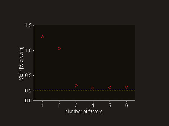
Figure 2. Set level SEP estimated using cross-validation as a function of the number of PLSR factors included in the NIR calibration model (o). The standard deviation of the reference value uncertainty is added as guide to the eye (---).
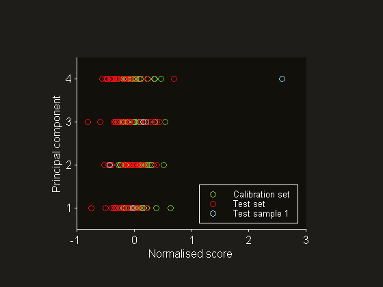
Figure 3. Normalised scores for principal components 1 through 4
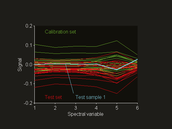
Figure 4. Mean-centred reflectance spectra digitised at six wavelengths between 1680 and 2310 nm.
Multivariate SEP at the global set level
Current practice is to characterise multivariate SEP at the set level. An SEP value is calculated as the root mean square (RMS) difference between predictions and reference values. It is important to stress that this procedure is only sound provided that the noise in the reference values is negligible compared with the true prediction uncertainty. The reason for this is that prediction errors are defined with respect to the true quantities, rather than noisy reference values. Consider the ideal situation where one has the perfect model and noisy reference values—a mental experiment. Of course, this example is not practical, but adding noise to the reference values as described by DiFoggio1 and Coates5 can always approach it to some extent. Clearly, the predictions should be perfect and the only contribution to SEP would originate from the measurement error in the reference values. In this extreme case, SEP would just estimate the standard deviation of the measurement error—it would not relate to the true prediction uncertainty at all! Thus, in general, the presence of this spurious error component leads to a so-called apparent SEP:1
\[{\rm{apparent }}SEP = {\left[ {(1/{n_{\rm{t}}})\sum\limits_{i = 1}^{{n_{\rm{t}}}} {{{({{\hat y}_i} - {y_{{\rm{ref,}}i}})}^2}} } \right]^{{\rm{\raise.5ex\hbox{$\scriptstyle 1$}\kern-.1em/ \kern-.15em\lower.25ex\hbox{$\scriptstyle 2$} }}}}\]
(1)
where nt denotes the number of samples in the test set, y^i is the prediction of property y for sample i (i = 1, …, nt) and yref,i is the associated reference value. The effect of the spurious error component is observed in Figure 2, which summarises the PLSR factor selection using cross-validation: the standard deviation of the reference value uncertainty (sref = 0.2%) is a lower bound for the SEP estimate. Similar plots abound in the multivariate calibration literature. The common plot of reference value versus prediction gives a graphical illustration of Equation (1), see Figure 5. It is clear that Equation (1) is equivalent to interpreting the deviation of the points from the “ideal” line entirely in the vertical direction. However, the foregoing discussion shows that the true prediction errors can be confounded to a large extent by measurement errors, which lie in the horizontal direction. In other words, the interpretation of such a plot is not always straightforward. The model could predict far better than one infers from the apparent prediction errors.
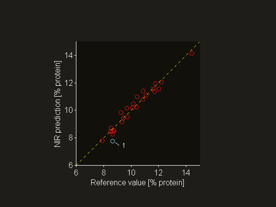
Figure 5. Reference value versus NIR prediction (o). For many samples the deviation from the “ideal” line with slope unity (---) is to a large extent due to the reference value uncertainty (sref = 0.2% protein), i.e. the deviation is not entirely a vertical one. Test sample 1 forms an exception: it has a relatively large (true) prediction error because it is an outlier.
A simple but effective correction for the spurious error component leads to1
\[{\rm{corrected }}SEP = {\left[ {{\rm{apparent }}SE{P^2} - s_{{\rm{ref}}}^{\rm{2}}} \right]^{{\rm{\raise.5ex\hbox{$\scriptstyle 1$}\kern-.1em/ \kern-.15em\lower.25ex\hbox{$\scriptstyle 2$} }}}}\]
(2)
where sref is an estimate for the precision of the reference method. This standard deviation is conveniently estimated as the standard error of laboratory (SEL) from a series of repeated measurements. Clearly, application of Equation (2) will always lead to an improvement in the sense that the corrected SEP is smaller than the conventional estimate obtained using Equation (1). Since apparent SEP also contains the inherent variability of the NIR methodology, it should, ideally, be larger than sref. However, the corrected SEP can only be properly estimated in practice if representative values for the apparent SEP and sref are available. Imprecise estimates can, for example, lead to the odd situation where apparent SEP < sref and the correction is not feasible. Obviously, sufficient experimentation is the price to be paid for obtaining a sharper SEP estimate.
Sørensen2 has documented a sizeable improvement for a number of NIR applications. It is important to note that one should not insert a pessimistic estimate for sref in Equation (2), because that would lead to an optimistic estimate for average prediction uncertainty. Finally, there is no reason why the corrected SEP could not be smaller than sref. Thus, Equation (2) shows that NIR predictions can, on average, be more precise than the reference values used for building the model, a fact that has been aptly illustrated by the noise addition experiments of DiFoggio1 and Coates.5
Multivariate SEP at the individual sample level
Characterising prediction uncertainty on the set level is the only way to answer important questions like “how good is my calibration?” It is therefore logical, for example, to monitor changes in the (set level) SEP when optimising a calibration model (spectral pre-treatment, factor selection etc.). However, as explained before, this procedure does not lead to sample-specific prediction intervals with good coverage probability. The American Society for Testing and Materials (ASTM) has recognised the need for a sample-specific SEP (E1655: Standard Practices for Infrared Multivariate Quantitative Analysis) and recommends the use of the following expression:
\[s({\hat y_i} - {y_{{\rm{ref,}}i}}) = {\left[ {(1 + {h_i}) \cdot SE{C^{\rm{2}}}} \right]^{{\rm{\raise.5ex\hbox{$\scriptstyle 1$}\kern-.1em/ \kern-.15em\lower.25ex\hbox{$\scriptstyle 2$} }}}}\]
(3)
where hi symbolises the leverage for sample i, SEC stands for the standard error of calibration and the remaining symbols are as defined under Equation (1). The leverage is related to the distance of a sample to the mean of the calibration set data. The calculation of SEC is similar to the calculation of the apparent (set level) SEP, i.e. Equation (1), but now one has to account for the degrees of freedom of the calibration model. Because SEC is explicitly based on reference values, Equation (3) leads to an apparent sample-specific SEP when the reference method is imprecise. In other words, Equation (3) is the sample-specific analogue of Equation (1). Obviously, the correction Equation (2) can also be applied on the sample level, leading to3
\[s({\hat y_i} - {y_{{\rm{true,}}i}}) = {\left[ {(1 + {h_i}) \cdot SE{C^{\rm{2}}}{\rm{ - }}s_{{\rm{ref}}}^{\rm{2}}} \right]^{{\rm{\raise.5ex\hbox{$\scriptstyle 1$}\kern-.1em/ \kern-.15em\lower.25ex\hbox{$\scriptstyle 2$} }}}}\]
(4)
where ytrue,i is the true value of property y for sample i. This formula has been used to calculate the sample-specific SEPs displayed in Figure 6. Figure 6 visualises that for the current NIR calibration 21 predictions (out of 26) are more precise than the reference value. In particular, the prediction for test sample 5 is more precise by almost a factor of 2. Likewise, this plot illustrates two drawbacks of the (set level) SEP as an uncertainty estimate for all future predictions. First, it does not differentiate between individual samples. Second, owing to the spurious error component of the reference method it often grossly overestimates the true prediction uncertainty. The preceding results imply that an adequate measure of prediction uncertainty is obtained when using Equation (4). Unfortunately, this claim cannot be directly verified by observations, because true reference values are not available. Consequently, one must resort to an indirect test. It is easily verified that a suitable indirect test is obtained by calculating an “expanded” SEP using Equation (3). This procedure leads to the expanded prediction intervals plotted in Figure 7. One expects 5% × 26 = 1 reference value to lie outside these expanded intervals, while the critical t-value is exceeded for test samples 3 and 6. Considering that it is only slightly exceeded for test sample 6 (2.12 against 2.09), one may infer that the interval provides correct coverage for the current data set. For other promising results, see Fernández Pierna et al.3
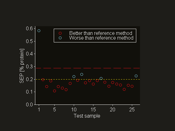
Figure 6. A comparison of sample-specific SEPs (o), the standard deviation of the reference value uncertainty (---) and the apparent set level SEP (— —). Note the exceptionally large (sample-specific) SEP for the outlying test sample 1.
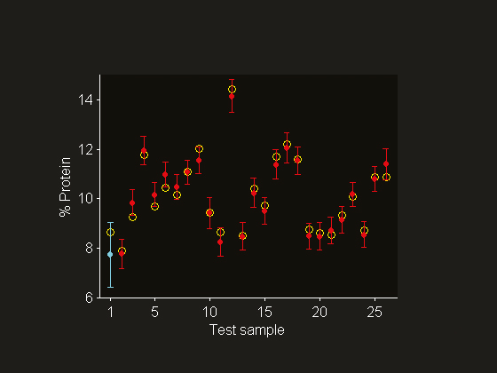
Figure 7. Reference values (o) and predictions (•) with 95% prediction interval. The error bars are calculated by incorporating the standard deviation of the reference value uncertainty (sref = 0.2% protein) into the sample-specific SEPs. Note that the outlying test sample 1 is contained in the expanded prediction interval.
Concluding remarks
In a formal sense, calibration model validation requires error-free reference values. In the rather common not-so-error-free situation, one should try to employ an estimate of the reference value uncertainty to correct for its adverse effect. The benefit of such a correction is that it always leads to sharper prediction uncertainty estimates, e.g. narrower prediction intervals. Laasonen et al. have recently published a thorough validation of a NIR method for determining the caffeine concentration in a pharmaceutical product.6 This work could easily be taken a step further by considering sample-specific uncertainty estimates. Finally, it is stressed that the proposed methodology is, in principle, not restricted to NIR calibration. Whereas the correction on the global set level is clearly independent of data and calibration method, the reasoning behind Equation (4) suggests that it should be suitable for other types of spectroscopy and calibration methods that are similar to PLSR.3 Application of Equation (4) to the calibration of excitation emission fluorescence data using multiway PLSR is currently under active research (R. Bro, Å. Rinnan, N.M. Faber, in preparation).
References
- R. DiFoggio, Appl. Spectrosc. 49, 67 (1995). https://doi.org/10.1366/0003702953963247
- L.K. Sørensen, J. Near Infrared Spectrosc. 10, 15 (2002). https://doi.org/10.1255/jnirs.317
- J.A. Fernández Pierna, L. Jin, F. Wahl, N.M. Faber and D.L. Massart, Chemom. Intell. Lab. Syst. 65, 281 (2003). https://doi.org/10.1016/S0169-7439(02)00139-9
- T. Fearn, Appl. Stat. 32, 73 (1983). https://doi.org/10.2307/2348045
- D.B. Coates, Spectrosc. Europe 14, 24 (2002).
- M. Laasonen, T. Harmia-Pulkkinen, C. Simard, M. Räsänen and H. Vuorela, Anal. Chem. 75, 754 (2003). https://doi.org/10.1021/ac026262w