A.M.C. Davies
Norwich Near Infrared Consultancy, 75 Intwood Road, Cringleford, Norwich NR4 6AA, UK. E-mail: [email protected]
Tom Fearn
Department of Statistical Science, University College London, Gower Street, London WC1E 6BT, UK. E-mail: [email protected]
Introduction
This column has been developed from two recent publications by Tom.1,2 My thanks to NIR Publications for allowing us to use Reference 1 essentially unchanged.
Tony
It is common practice in near infrared (NIR) calibration to apply pre-treatments designed to correct for the scatter effects usually seen in absorbance data. These pre-treatments can interfere with interpretation of the spectra. This is illustrated here with the aid of two rather extreme artificial examples.
Example 1
Figure 1 shows three mathematically created absorbance spectra. In the regions where only one spectrum can be seen it is because the three spectra are coincident.
The spectra were created by adding two Gaussian peaks to a zero-level baseline. The first peak, centred on wavelength 30, is identical in all three spectra. The second, centred on wavelength 70, is different in each spectrum. In this idealised example this variable peak represents the absorbance of the analyte of interest, the concentration of which is supposed to vary in the three samples. If these spectra were observed, interpretation would be straightforward, and the correct conclusion would be drawn.
In Figure 2 the spectra of Figure 1 have been subjected to some scatter effects, again in an idealised mathematical manner. Different horizontal baselines have been added to the three spectra, and a different multiplicative scaling has been applied to each one. Now both peaks vary in height, because of the effect of the different scaling, and the interpretation is much less clear. This, unfortunately, is the typical situation with NIR spectra.


The usual remedy for this problem is to apply a pre-treatment designed to correct for scatter effects. Since the transformation that converted the spectra of Figure 1 into those of Figure 2 was a baseline shift and a multiplicative scaling, one might hope that either the standard normal variate (SNV)3,4 or multiplicative scatter correction (MSC)4,5 pre-treatments, both of which shift and scale the spectra, might undo these idealised scatter effects.
Figures 3 and 4 show the results of applying SNV and MSC, respectively. The effects of the two treatments are, as is often but not always2 the case, very similar. This common effect, though, is not the desired one. After pre-treatment it is the first peak, which was constant in the original spectra, that shows variation, and the second peak, which originally varied, that is now almost constant. The obvious interpretation from either of Figures 3 or 4 would be incorrect, assigning the wrong peak to the analyte.


Discussion of Example 1
Naturally the artificial example was constructed with the deliberate intention of achieving this disturbing result. The key is in the relative sizes of the peaks. SNV tries to make the vertical range more or less the same for all the spectra, while MSC applies shift and scale factors that try to make the treated spectra coincide as far as possible. Both criteria are optimised by scaling the large peaks so that they coincide, and so this is precisely what both pre-treatments do.
The point of the example is not to suggest that we should not be using these pre-treatments. They are valuable tools for removing unwanted variability and helping to make calibrations more robust. The point is to warn that these pre-treatments, along with others that shift or rescale spectra in a simple fashion, have the potential to lead to erroneous interpretations. An effect as dramatic as that shown here is unlikely to occur in practice, but there will always be a tendency for information in one wavelength region to be shifted elsewhere or simply smeared across the whole wavelength range. If the spectra in Figures 3 and 4 were used in a PLS or PCR calibration, the first peak would show up strongly in both loading and coefficient vectors. This is yet another reason to be cautious in interpreting these vectors in situations where we do not already have a good idea which are the important absorbances.6
Example 2
In the discussion of Example 1 you should have noticed the warning “... but not always ...”. MSC and SNV are different transformations so sometimes they can produce different and important modifications of spectra. Probably none as spectacular as in this second example utilising different artificial data.
If we have a “spectrum” measured at only three wavelengths then we can draw diagrams to show the transformation. Figure 5 shows some artificial spectral data, computed by a random number generator. The magenta, circular points represent 21 raw, i.e. untreated, spectra, each measured at three wavelengths, and plotted in a space with one dimension corresponding to each wavelength.

The result of applying SNV to this data is shown in Figure 6 while that for MSC is shown in Figure 7. How can they possibly be so different? Figures 8–10 show what happens.
SNV transformation
SNV3,4 transforms each spectrum by subtracting a mean and dividing by the standard deviation of the measured values.
The first step for both SNV and MSC transformations, subtraction of the mean, can be visualised as a projection of the 21 points onto a orthogonal planar subspace, as shown in Figure 8.

The thick line shows a vector whose origin and direction are defined by the cross and the yellow plane on which it lies. Any vector lying in this plane has mean of zero. Geometrically, subtracting the mean corresponds to projecting the points representing raw spectra orthogonally onto the plane, where the result is shown as a cyan circle.
The second step for SNV, division by the standard deviation, is shown in Figure 9.

This is the plane of Figure 8, with the cyan circles representing the projected (mean-centred) spectra and the cross in the centre the origin. After dividing by the standard deviation all the spectra have the same length. The orientation is preserved, so the scaled spectra are now the points represented by blue circles in the figure. This is how the circular structure is produced. Thus with our three wavelengths, all the SNV treated spectra will all be found on this circle, as shown in Figure 6. Generally, we have far more than three wavelengths and it would be very surprising to see the full circle, as in the artificial example of Figure 6. This is because we would normally be processing spectra which have a large degree of similarity. In these normal cases the spectra will only be projected on to a small part of the potential circle so usually the curvature will not be seen.
MSC transformation
MSC4,5 transforms each spectrum by subtracting an intercept, a, and dividing by a slope, b. a and b are computed as the intercept and slope of a least-squares regression of the values of the spectrum on the corresponding values of a reference spectrum. Usually this reference spectrum is the mean spectrum in a calibration set. The geometry of this subtraction is very similar to Figure 8. The only difference is that SNV treated spectra all have a mean of zero, while MSC treated spectra have the same mean as the reference spectra. This is achieved geometrically by moving the yellow plane until the reference spectrum lies in it, the orientation is unchanged.
The second step, division by b, is shown in Figure 10.

Figure 10, like Figure 9, is the yellow plane from Figure 8 but this time showing the second stage of MSC. The cyan circles, which have the same configuration as in Figure 8, are the spectra after subtraction of the intercepts, and the red circles are the same spectra after scaling by b. The solid green circle represents the reference spectrum, which is connected to the origin by a thick line. When scaling by b the orientation of each spectrum is preserved so that it still lies on the same line through the origin, but it is moved along this line until its projection onto the direction of the reference spectrum is exactly equal to the reference spectrum. The result is that the red circles all lie on the straight line that passes through the reference spectrum and is orthogonal to the line joining it to the origin. To achieve this result, some of the lines need to be extrapolated beyond the origin and some of them with slopes close to zero (positive or negative slopes) may need to be extrapolated a long way. These points are seen as outliers.
Discussion of Example 2
It did require very extreme data to produce these results. However, it should be noted that this data is not a freak result; it is because the data is random. The same result was obtained with a different set of random data in the original publication.2 The curvature will often be seen at high dimensions in data treated by SNV and some of this may be retained when compressing to lower dimensions. MSC will tend to emphasise outliers more than SNV and MSC treated spectra may tend to contain a few more outliers than with some other pre-treatments.
The point of showing you these examples is to emphasise that these are different transformations and one or the other will occasionally produce a better performance with a given set of spectra but very occasionally produce very strange plots.
References
- T. Fearn, “The effect of spectral pre-treatments on interpretation”, NIR news 20(6), 15 (2009).
- T. Fearn, C. Riccioli, A. Garrido-Varo and J.E. Guerrero-Ginel, “On the geometry of SNV and MSC”, Chemometr. Intell. Lab. Syst. 96, 22 (2009).
- R.J. Barnes, M.S. Dhanoa and S.J. Lister, “Standard normal variate transformation and detrending of near infrared diffuse reflectance spectra”, Appl. Spectrosc. 43, 772 (1989).
- T. Næs, T. Isaksson, T. Fearn and T. Davies, A User Friendly Guide to Multivariate Calibration and Classification. NIR Publications, Chichester, Chapter 10 (2002).
- P. Geladi, D. McDougall and H. Martens, “Linearisation and scatter correction for near infrared reflectance spectra of meat”, Appl. Spectrosc. 39, 491 (1985).
- T. Fearn, “Interpreting coefficient vectors”, NIR news 19(6), 15 (2008).
Computational chemistry
We had some enthusiastic responses to the column on computational chemistry and we will be following this up in 2010. I would be pleased to hear from any spectroscopists who make use of computational chemistry in their work.
Tony Davies