A.M.C. Davies and Tom Fearn
Norwich Near Infrared Consultancy, 75 Intwood Road, Cringleford, Norwich NR4 6AA, UK. E-mail: [email protected]
Department of Statistical Science, University College London, Gower Street, London WC1E 6BT, UK. E-mail: [email protected]
More “Back-to-basics”
In December 2004 I made the decision that this column should make a return visit to topics in quantitative analysis that had been covered (or sometimes just mentioned) in previous columns. Within seconds of that decision I realised that we would need to treat qualitative analysis to the same revision. The quantitative aspects turned out to be a three year marathon* journey but we have at last arrived at the start of what was conceived as “Part 2”.
I have been working on problems in qualitative analysis for 40 years! That’s before chemometrics as a topic began and I regard them as being much more demanding than quantitative analysis. There are several reasons for this, some more obvious than others:
- qualitative analysis is not a single problem,
- some humans are very good at looking at spectra and making qualitative decisions,
- solutions require more statistics than are needed for quantitative analysis.
Problems in qualitative analysis
From the classical point of view, qualitative analysis is divided into supervised or unsupervised methods but the number of different objects is also very important. The question “Is this sample compound A or compound B?” is different to the question “Is this sample compound A, or B, or C, or ..., or Z” and very different to the request “Identify this sample”.
Human skills
Spectroscopists have been looking at spectra, and giving answers to all three types of questions listed above, for a very long time. I do not know of any spectroscopists who would claim to be able to look at a spectrum and estimate the percentage of ingredient x, but computers can, so qualitative analysis must be a less difficult problem!
A recent query from one of our readers (always welcome!) resulted in an e-mail discussion with some of the world experts on IR qualitative analysis. Their view is that qualitative analysis is too difficult to trust to a computer! As Peter Griffiths points out in his recent second edition of Fourier Transform Infrared Spectrometry, “... a library search cannot identify an unknown unless the unknown is present in the library”.1
Statistics in qualitative analysis
In quantitative analysis if we have the RMSEP then we have all the statistics we need (some others may be useful). In qualitative analysis we need to know standard errors but we also need to know about distance measures, decision boundaries, prior probabilities, misclassification costs, ... . Luckily for me I have had Tom Fearn to guide and advise me for the last 25 years and most of what follows is Tom’s work, much of it previously published in the “Chemometric Space” in NIR news2 or in our frequently referenced book.3
Tony Davies
Supervised and unsupervised classification
Statistical classification has a number of interesting applications in spectroscopy. For NIR data in particular, it has been used in a number of scientific publications and practical applications.
There is an important distinction between two different types of classification: so-called unsupervised and supervised classification. The former of these usually goes under the name of cluster analysis and relates to situations with little or no prior information about group structures in the data. The goal of the techniques in this class of methods is to find or identify tendencies of samples to cluster in sub-groups without the use of any prior information. This is a type of analysis that is often used at an early stage of an investigation, to explore, for example, whether there may be samples from different sub-populations in the dataset, for instance different varieties of a grain or samples of chemicals from different suppliers. In this sense, cluster analysis has similarities with the problem of identifying outliers in a quantitative data set.
Cluster analysis can be performed using very simple visual techniques such as PCA, but it can be done more formally, for instance by one of the hierarchical methods. These are techniques that use distances between objects to identify samples that are close to each other. The hierarchical methods lead to so-called dendrograms, which are visual aids for deciding when to stop a clustering process.
The other type of classification, supervised classification, is also known under the name of discriminant analysis. This is a class of methods primarily used to build classification rules for a number of pre-specified subgroups. These rules are later used for allocating new and unknown samples to the most probable sub-group. Another important application of discriminant analysis is to help in interpreting differences between groups. Discriminant analysis can be looked upon as a kind of qualitative calibration, where the quantity to be calibrated for is not a continuous measurement value, but a categorical group variable. Discriminant analysis can be done in many different ways, some of these will be described in following columns. Some of the methods are quite model orientated, while others are very flexible and can be used regardless of structures of the sub-groups.
Some of the material in earlier columns on quantitative analysis is also relevant to classification. Topics and techniques such as collinearity, data compression, scatter correction, validation, sample selection, outliers and spectral correction are all as important for this area as they are for quantitative calibration.
Distance measurements used in classification
It seems a good idea before we begin a discussion of techniques to describe some of the ways of measuring distance that we will be using. The message is that there are some very simple though perhaps non-obvious relationships between some of these measures.
Spectra as vectors
A spectrum x = (x1, x2, ..., xp) measured at p wavelengths can be thought of as a point in p-dimensional space by taking each of the p measurements as the coordinate in one of the dimensions. We may equally well think of the spectra as vectors, by joining the point representation of the spectrum to the origin with a line. As usual, the trick to understanding the maths is to consider the case p = 3, for which it is easy to draw the picture. Figure 1 shows two vectors in a three-dimensional space.
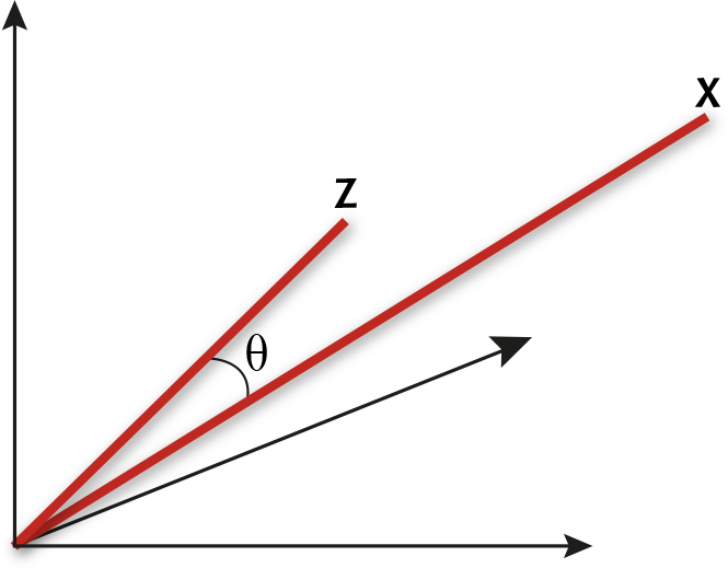
Two spectra as vectors c and z in a three-dimensional space
Euclidean distance
Euclidean distance, D, is the “natural measurement” of distance between two objects.
Geometrically, D is the length of the line joining the ends of the two vectors in the figure. For the multi-dimensional case it is defined as:
D2 = (x1 - z1)2 + (x2 - z2)2 + ... + (xp - zp)2
= S(xi - zi)2
which expands to:
D2 = S xi2 + S zi2 – 2 S xi zi
Angles between vectors
Geometrically, we can just measure the angle q between the two vectors in Figure 1. If the vectors represent spectra, then we can call this the angle between the spectra. It is clear from the picture that the more similar the two spectra, the closer together will be the two points and the smaller will be the angle between the corresponding vectors. Of course it is usually preferable to use a formula to compute the angle between x = (x1, x2, ..., xp) and z = (z1, z2, ..., zp) directly from the measurements. The relevant formula is the one that relates the so-called dot product of the two vectors
x.z = x1 z1 + x2 z2 + ... + xp zp = S xi zi
to their lengths |x| and |z| and the angle q between them. The formula is
x.z = |x| |z| cos q (1)
where
|x|2 = x12 + x22 + ... + xp2 = S xi2
and
|z|2 = z12 + z22 + ... + zp2 = S zi2
Thus, to compute the angle we compute the dot product and the two lengths, and then use Equation (1) to find cos q, and hence q.
Standardising the length
If we are going to be computing a lot of these angles, it makes sense to standardise all the spectra so that each has length 1. This is achieved for x by dividing each xi by |x|.
In the picture, the vectors keep their direction but are rescaled in length to lie on a sphere of radius 1. Then |x| = |z| = 1 and Equation (1) reduces to
x.z = cos q (2)
Now the angle and the dot product are equivalent measures of distance in the sense that each can be calculated simply from the other. Note though that the maximum dot product, 1, corresponds to the minimum angle, 0, whilst a dot product of 0 corresponds to an angle of p/2 = 90°. This equivalence means that we could equally well define a region of similarity around x as all spectra that have a dot product with x exceeding d, or as all spectra that make an angle of less than cos–1 d with x.
Relation with Euclidean distance
Using standardised spectra, there is a fairly simple relation between these two measures and the Euclidean distance D.
If D2 = S xi2 + S zi2 – 2 S xi zi
then when the vectors are standardised and the first two terms are each 1, we have
D2 = 2(1 - x.z) = 2(1 - cos q)
Thus, for standardised spectra, the dot product, angle and Euclidean distance are all three equivalent measures of distance. A region of similarity defined by any of the three would be all spectra that lie within a circle around x on the surface of the sphere.
The dot product is easily the quickest to calculate, so would be the preferred measure from a computational point of view. For non-standardised spectra the three measures would, of course, all be different.
Relation with correlation
Another measure sometimes used to compare spectra is the correlation coefficient between them. To relate this to the distance measures above we need to centre as well as scale the spectra. Suppose we transform from x to x*, where the ith element xi* of x* is given by
xi* = (xi - mx) / lx (3)
where
mx = S xi / p
is the mean of the elements in x and
lx2 = S(xi - mx)2
is the squared length of x after it has been centred. Then the dot product between x* and the similarly centred and scaled z* is
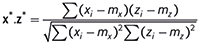
which, by definition, is the correlation coefficient between x and z. Thus we have yet another equivalence: the correlation is the same as the dot product if we centre and scale the spectra before computing the latter.
The transformation in Equation (3) looks rather similar to the well-known SNV standardisation.4,5 The only difference is that SNV would normally use sx as a divisor rather than lx, where
sx2 = lx2 / (p - 1)
The only difference this would make is that the dot product now becomes p - 1 times the correlation. This does not change the fact that the two are equivalent, it just introduces a scale factor into the equation relating them. Thus, in this sense, using the correlation coefficient (or its square) as a distance measure is essentially the same as pretreating with SNV and using either the angle or the dot product between the spectra as the distance measure.
References
- P.R. Griffiths and J.A. de Haseth, Fourier Transform Infrared Spectrometry, 2nd Edn. John Wiley & Sons, Inc. Hoboken, NJ, USA (2007). https://doi.org/10.1002/047010631X
- T. Fearn, NIR news 14(2), 6–7 (2003).
- T. Næs, T. Isaksson, T. Fearn and T. Davies, A User-Friendly Guide to Multivariate Calibration and Classification. NIR Publications, Chichester, UK (2002).
- J. Barnes, M.S. Dhanoa and S.J. Lister, Appl. Spectrosc. 43, 772 (1989). https://doi.org/10.1366/0003702894202201
- A.M.C. Davies and T. Fearn, Spectrosc. Europe 19(6), 15 (2007). https://www.spectroscopyeurope.com/td-column/back-basics-final-calibration