Carlos Cobas,a Felipe Seoane,a Santiago Domínguez,a Stan Sykorab with Antony N. Daviesc
aMestrelab Research SL, Feliciano Barrera 9B Bajo, Santiago de Compostela, Spain
bExtra Byte, Castano Primo, Italy
cProfessor of Analytical Science, SERC, University of Glamorgan, UK, and Director, Analytical Laboratory Informatics Solutions
Introduction
Simple proton nuclear magnetic resonance (1H NMR) experiments still remain the most widely used NMR analytical technique despite the phenomenal advances in the design of more sophisticated experiments, with new pulse sequences continuously emerging. It is the most sensitive, fastest and is very information rich providing valuable structural information. The spectra are usually interpreted by hand, primarily considering chemical shift, intensities and coupling constants. This manual process is very time consuming, and can become a process bottleneck in fields such as high-throughput NMR. The more widespread deployment of new instrumentation, including automatic sample changers and flow probes, has also enabled the acquisition of NMR spectra of even larger numbers of compounds.1 Greater automation of the spectral analysis process has become essential if NMR is to be of value as a high-throughput analytical method in the future.
Traditional computer assisted analysis of 1H NMR spectra followed two different approaches: Quantum Mechanical (QM) spin system calculation and iterative optimisation of the spectral parameters.2 This is certainly the most rigorous yet complex method, but interestingly, the most popular approach even more than 40 years ago3,4,5 when computer power was very limited.
The second approach, which incidentally has attracted significant interest in recent years despite being computationally less demanding than the previous method, is based on the same technique typically used by most organic chemists, i.e. on the use of the popular first-order analysis rules.6,7,8,9,10,11 This approach is only valid in weakly coupled systems and, thus, has a more limited scope when compared to QM methods, but is useful for a rapid spectrum analysis.
Regardless of the method employed, the main obstacle to achieving a successful automatic analysis of 1H NMR spectra with minimal user intervention lies in the fact that NMR spectra are not only spectral peaks arising from the transitions of the studied spin system, but also many others, such as, solvent and impurity peaks, spinning sidebands, reference peaks (e.g. TMS), satellite peaks from the very same spin system(s) isotopomers and labile peaks. Identification of any obvious impurities or solvents is a task an experienced chemist is very familiar with, but extremely difficult for a computer program. These peaks can overlap with compound resonances, making some simple strategies based on the definition of “solvent” regions ineffective.
This column addresses the application of Global Spectral Deconvolution (GSD) for computer assisted analysis of 1H NMR spectra of small molecules. GSD can be used to classify peaks in a spectrum according to their origin (i.e. compound peaks versus artefacts). The resolution enhancement power and the automatic determination of the number of nuclides in a spectrum by GSD will also be discussed.
Global Spectral Deconvolution
GSD is a complex algorithm and a brief summary of GSD’s theory and implementation will be provided here in the context of automatic analysis of 1H NMR spectra.
GSD is conceptually very simple: it automatically reduces a frequency domain spectrum to a set of Lorentzian or near Lorentzian lines leaving out any baseline drift and noise. The output of GSD is a ‘‘peak list’’ of spectral parameters for Lorentzian lines in terms of frequency, amplitude, line width and, optionally, phase of all the desirable information present in the original spectrum but none of the superfluous “noise”. These peaks can then be subject to automatic and/or manual editing such as automatic recognition of spikes (anomalously narrow peaks), solid impurities (very broad peaks), folded-over peaks (anomalous phase), rotation sidebands and isotopomer satellites. All subsequent data processing tasks (such as integration, multiplet analysis or structure verification and/or elucidation) can work exclusively on this clean numeric information.

An example of GSD in action is illustrated in Figure 1, which shows the spectrum of Santonin {(3S,5aS)-3,5a,9-trimethyl-3a,4,5,5a-tetrahydronaphtho[1,2-b]furan-2,8(3H,9bH)-dione} recorded in deuterated chloroform with TMS as reference at 800 MHz. All individual peaks deconvolved by GSD and the synthetic sum of those GSD peaks are shown superimposed with the experimental spectrum. Peaks are colour coded—compound (green), solvent (red) or reference peaks (TMS, brown). This assignment is carried out automatically by a fuzzy logic expert system although manual assignment is also allowed.
In order to achieve this level of automation, a method was devised capable of correctly defining the total number of spectral peaks present in the spectrum prior to any fitting.
A reliable calculation of the derivatives is especially important, particularly in spectra with poor signal-to-noise ratio. An enhanced version of the Savitsky–Golay convolution algorithm12 is used where the number of points and order are calculated automatically. The use of derivatives all but removes any baseline dependence. Moreover, the use of the second derivative enormously enhances resolution and converts bare shoulders into distinct peaks. This can be appreciated in the inset of Figure 1, which shows a multiplet with peaks with a significant grade of overlap and where GSD successfully recognises all peaks. Another example of the resolution power of GSD is depicted in Figure 2 which shows what it seems at first glance is a double doublet (experimental peaks are shown in red) whereas GSD detects a total of eight peaks. Complete analysis of the spectrum with its corresponding molecule confirmed the results obtained with GSD.

Another example showing the potential of GSD selectively to suppress any unwanted signals and therefore to enable automatic extraction of accurate NMR integrals, even when the peaks of interest are heavily convoluted with other solute or solvent resonances, is illustrated by examining a region of an estradiol {[17b]-Estra-1,3,5(10)-triene-3,17-diol; Scheme 1} 1H NMR spectrum acquired in DMSO-d6 containing a broad water peak that overlaps and interferes with the 13-H multiplet. Figure 3(b) shows this spectral region in the original data. Buried under the broad HDO peak is a triplet whose presence and area are important for the correct spectral to structure validation.

 Original raw spectrum (b) Region of interest containing the DMSO and HDO peaks overlapping the 13-H triplet. (c) Result of applying GSD. Green lines correspond to the individual deconvolved peaks labelled as compound resonances whereas red peaks are automatically assigned as solvent peaks (d) GSD-derived spectrum resulting after removal of solvent resonances.")
Figure 3(c) shows the result of applying GSD to the original spectrum. It can be seen that GSD identifies and deconvolves correctly the triplet obscured by the large H2O peak. Figure 3(d) shows the resulting GSD-derived spectrum synthesised without the solvent peaks and using the original line widths as derived from the deconvolution process. The integrals calculated from this synthetic spectrum match the expected stoichiometry of the structure. Clearly, any evaluation method employing only exclusion areas (sometimes referred to as dark regions) would fail in the analysis of this spectrum as the triplet would be missed.
Automatic solvent–recognition
For a successful automatic analysis of 1H NMR spectra it is of vital importance that solvent peaks are identified prior to any further evaluation being carried out. At first glance, this seems like a trivial task as the chemical shifts of most common solvent peaks are relatively well known in advance.13
In practice, however, reliable automatic identification of signals deriving from common solvents is a tremendously challenging task for an automatic computer algorithm due to a number of reasons. Without going into a detailed discussion, the one important issue to take into account is the noteworthy chemical shift dependence on experimental conditions (e.g. concentration, temperature, pH etc.). In particular, it is important to note that the chemical shift of water as a secondary solvent is quite temperature-dependent and any potential hydrogen bond acceptor will tend to shift the water signal from its expected position, sometimes by several ppm. Another tricky problem in the case of water is that it does not only show up as a singlet but also as a more complex multiplet presenting a convoluted fine structure. For example, the water peak shown in the inset of Figure 1 is actually comprised of three peaks. Depending on the experimental conditions and on the solute, the water peak can appear in many different forms, line widths and chemical shifts, complicating its automatic detection.
Even worse—some of the solvent signals overlap with resonances of the compound. Examples of this problem have already been shown in Figures 1 and 3.
To resolve these issues a fuzzy-logic expert system for the recognition of the solvent signals in a spectrum was developed. For each solvent multi-multiplet structure (MMS), the system scores every GSD peak against a number of properties listed in a special spectral solvent descriptor, trying to estimate whether the selected peak could be the pivot line of the MMS. The peak with the highest score, provided it exceeds a certain threshold, is then accepted as the pivot and, working backwards, all recognisable peaks of the MMS are labelled as solvent. Some of the parameters included in the scoring system are the expected chemical shift, line width, amplitude, multiplicity, HD coupling constant, secondary multiplet, 13C satellite multiplets etc. For example, the primary MMS pattern for DMSO is composed of 18 peaks! The scoring system assigns different scores and significances to each individual parameter.
Some examples of the performance of the solvent detection scoring system can be seen below.
 and a vertical expansion to show the 13C satellites (blue signals).")
In Figure 4 the aromatic region of the strychnine spectrum in chloroform is depicted. It can be seen that the solvent peak is a tricky one to label properly since it appears accidentally perfectly overlapped with one of the peaks of proton H-14 (see Scheme 2).

In this case, the system found 13C satellites (blue peaks in Figure 4, right) which give a significant premium to the scoring system when scoring for chloroform, and even though the chemical shift for this peak is slightly different to the expected value (7.20 ppm versus 7.26 ppm per Table in Reference 13), the overall result of combining all different descriptors in the scoring system yielded the correct identification of the solvent peak. It is worth pointing out that the detection of chloroform is generally more challenging than other solvent peaks (e.g. DMSO) as it is a singlet (apart from the 13C satellites), and therefore not susceptible to identification by the application of pattern recognition techniques.
The opposite case is that of the automatic detection of DMSO peaks, which can be facilitated by the fact that the multiplicity of its quintuplet (see Figure 5, left) can be exploited by the scoring system.

When the solvent presents a clear multiplet structure, like the quintuplet in DMSO, and is matched during the evaluation process, it results in a good premium in the multiplet pattern recognition test of the scoring system. The same applies if the isotopomer satellites are also matched (e.g. 13C satellites in DMSO, see Figure 5 right). However, this does not mean that it is absolutely necessary to find the 13C satellites or the five peaks in the DMSO. The system is flexible enough in such a way that if any of those properties are found, the probability that the signals under analysis correspond to a solvent peak will be higher, but if any of the individual scoring system tests fail, this does not preclude the solvent line being detected.

This flexibility is illustrated with the two examples depicted in Figure 6. The image on the left is shown as an example since the DMSO signal is immersed in a crowded area with many compound signals and therefore the 13C satellites are not detected. Despite this, the algorithm is capable of marking the solvent lines properly with high selectivity. In contrast, Figure 6 right shows an extreme case of poor resolution in which GSD is not able to resolve the fine structure of the DMSO peak, but in which the signal-to-noise ratio is good enough to extract the 13C satellite peaks. As a result, the algorithm also identifies the solvent peaks correctly.
Automatic determination of the number of nuclides
A basic principle of NMR is that the area of each signal in a spectrum is proportional to the number of nuclides contributing to the signal. Of course, in the context of structural analysis, what matters is the ratio of the integrals, not the absolute values, as they depend on instrumental conditions. Classically, one integral is selected and a number of nuclides assigned to it so that all remaining integrals will be normalised by the value of that reference integral. For a computer algorithm, the challenge rests in automatically finding the number of nuclides arising from a particular integral.
The combination of a Bayesian algorithm with GSD and the automatic detection of solvent and reference peaks proved to be very effective for the automatic identification of the correct integration values. In standard conditions of signal-to-noise ratio and purity, the automatic calculation of the number of nuclides works extremely well. This happens even in those cases in which solvent peaks are buried within multiplets of the compound, as in the examples shown in Figures 1 and 2. Another example is illustrated in Figure 7.

In a fully automated way, once GSD has been run and the peaks automatically flagged according to their type (compound, solvent etc.) and after automatic selection of the integral boundaries, the total number of nuclides for this spectrum is 27, a result compatible with the chemical structure (not shown here). Peaks identified as solvent are automatically skipped during the integration process. Furthermore, the multiplet at 3.46, which corresponds to two CH2, can be properly quantified despite the large overlapping water peak.
Conclusions
Once all non-compound signals, including impurities, solvent and reference peaks and other spectral imperfections have been purged out of the experimental 1H NMR spectrum, automatic analysis of 1H NMR spectra of small molecules becomes a much less challenging task. In particular, multiplet analysis using first order rules is much more efficient, especially in cases of severe signal overlap or multiplets contaminated with solvent peaks. For example, Figure 8 shows the result of analysing the spectrum of Santonin (same as in Figure 1) fully automatically (i.e. with one button click).

References
- P.A. Keifer, S.H. Smallcombe, E.H. Williams, K.E. Salomon, G. Mendez, J.L. Belletire and C.D. Moore, J. Comb. Chem. 2, 151–171 (2000).https://doi.org/10.1021/cc990066u
- P. Diehl, S. Sykora and J. Vogt, J. Magn. Reson. 19, 67 (1975).
- J.D. Swalen and C.A. Reilly, J. Chem. Phys. 37, 21 (1962).https://doi.org/10.1063/1.1732968
- S. Castellano and A.A. Bothner-By, J. Chem. Phys. 41, 3863 (1964).https://doi.org/10.1063/1.1725826
- D.S. Stephenson and G. Binsch, J. Magn. Reson. 37, 395 (1980).
- T.R. Hoye and H. Zhao, J. Org. Chem. 67, 4014–4016 (2002).https://doi.org/10.1021/jo001139v
- C. Cobas, V. Constantino-Castillo, M. Martín-Pastor and F. del Río-Portilla, Magn. Reson. Chem. 43, 843–848 (2005).https://doi.org/10.1002/mrc.1623
- S. Bourg, J.-M. Nuzillard, J. Chim. Phys. 95, 18 (1998).https://doi.org/10.1051/jcp:1998119
- L. Griffiths, Magn. Reson. Chem. 38, 444 (2000).https://doi.org/10.1002/1097-458X(200006)38:6<444::AID-MRC673>3.0.CO;2-Z
- L. McIntyre and R. Freeman, J. Magn. Reson. 96, 425 (1992).
- J. Stonehouse and J. Keeler, J. Magn. Reson. A 112, 43 (1995).https://doi.org/10.1006/jmra.1995.1008
- A. Savitzky and M.J.E. Golay, Anal. Chem. 36, 1627–1639 (1964).https://doi.org/10.1021/ac60214a047
- H.E. Gottlieb, V. Kotlyar and A. Nudelman, J. Org. Chem. 62, 7512–7515 (1997).https://doi.org/10.1021/jo971176v